|
|
|
|
It's a slippery slope that lies before us...
|
The next concept we need to put in our toolbox is the notion of
"rate of change". The example that most of us were
first exposed to was speed being the rate of change of distance.
My first science course, and probably yours as well, contained
the formula,
speed=distance/time.
This is the prototype of all rate of change formulae. In
general a rate of change may be the change in anything divided by
the corresponding change in a related variable. The
"slope" of a graph of y vs. x for example is the change
in y divided by the corresponding change in x. It is called the
rate of change in y with respect to x. Since we are going to be studying dynamical systems where time is normally taken to be the independent variable, we will make that the case in our examples.
Since t is the independent variable, we will pick two points
on the t-axis to be the interval over which we will calculate the
rate of change. The difference between these t values is called
"delta t". The upper case Greek letter delta (
D
) is used as a symbol of this finite difference.
Customarily we subtract the lower t value from the higher to get
D
t.
For each of the chosen t values
there will be a corresponding value of x. We get
D
x by subtracting the x corresponding with
the lower t value from that corresponding to the upper t value.
The ratio
D
x over
D
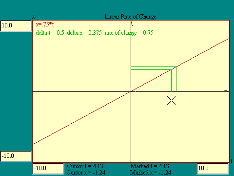
t is the rate of change, and for a straight line, the
slope of that line. Run the
Linear Rate of Change
display to experiment with this. I have chosen a
D
t of 0.5 units for this display You may
select the lower value of t using the cursor. The x cursor value
will be ignored. As you will see, the slope of a linear function
is a constant.
|
|
|
|
|
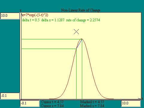
Now suppose that x is a nonlinear
function of t. Would that alter our idea of rate of change? In
the nonlinear case compare the rate of change at various
locations along the t axis. We will use the
Gaussian function
as a model of
a nonlinear function. Notice that the rate of change we get is
some sort of average rate of change over the interval. Run the
Non-Linear Rate of Change
display to try out this idea.
|
|
We will find it useful to be able to associate a rate of
change with a particular value of the independent variable. In
the linear case this is easy since the rate of change is constant
everywhere. In the nonlinear case we need to do some more
thinking about the situation. Not only does the rate of change
depend on where along the t axis we look, it also depends on how
we select the interval over which to measure it. Suppose we
looked at shorter and shorter intervals such that delta t was
smaller than any small number you could choose, approaching zero
itself. What would happen to the rate of change
D
x /
D
t. Run the
Infinitesimal Delta t
display to see.
What we saw happen in the last display was the rate of change
approaching a limit as
D
t got smaller and smaller. That limiting value is called the
"derivative" of x with respect to t at the value of t
picked for the left end of the
D
t interval. If we draw a line which just touches the curve at a
point, the slope of that line is the derivative of x with respect
to t at that point. Such a line is called a "tangent"
to the curve. The derivative of x with respect to t is written
dx/dt, symbolizing that it is the limiting value of
D
x over
D
t as
D
t approaches zero.
|

|
|
There are some assumptions about the nature of the function we
are working with which make possible this idea of letting
D
t approach zero and finding the limiting value of
D
x over
D
t. For this to work the function must be continuous,
meaning that there is an x for every real number t in the domain
of the function. And it must be smooth, meaning that as I look at
smaller and smaller
D
t, the absolute value of the corresponding
D
x also decreases continuously. There are some badly behaved functions
which do not meet these conditions but we will steer clear of
them.
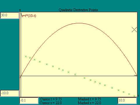
Now that we have defined the derivative of a function at a
point, we could calculate it for every point on a curve. Or at
least for enough points on a curve to get some idea what dx/dt
would look like as a function of t. Let's work with the
quadratic function.
Run the
Quadratic Derivative Points
display to do this.
The question comes up, if
x=10*t-t^2
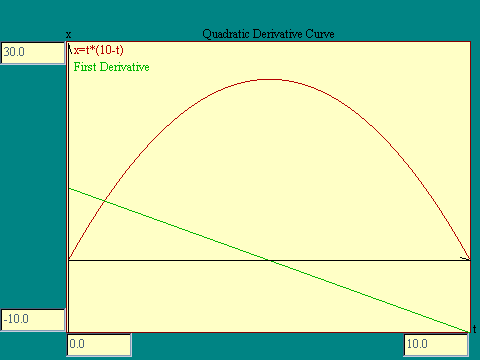
what is the function dx/dt. We have seen a graph of dx/dt in
the last display. It is a straight line cutting the x-axis at 10
and the t axis at 5. We know the equation of such a line from
basic algebra. It is
x=10-2*t .
If you experimented with a great many functions of form
x=a*t^n
you would discover that the derivative is always
n*a*t^(n-1) .
Verify that this formula gives the correct derivative of
x=10*t-t^2
noting that the derivative of a sum is the sum of the derivatives
and remembering that
t^0=1.
|
|
Here is how that verification we talked about above goes. The
function
x=10*t-t^2
has two terms in it, the 10*t and the -t^2. Applying the
n*a*t^(n-1) rule, 10*t^1 yields 1*10*t^(1-1) or 10*t^0 or 10. For
the second term -t^2 yields 2*(-1)*t^(2-1) or 2*t. Since the
derivative of a sum (10*t)+(-t^2) is the sum of the derivatives,
d(10*t-t^2)/dt = 10-2*t
as required. Replacing the few points plotted in the image above with the line whose equation we just derived, we get the results shown at the right.
|
|
|
The derivative of many different functions have been studied
and the form of the derivative tabulated. Also there are rules
for how the derivatives of composite functions are to be
calculated from the derivatives of basic functions. An example of
this was my statement that the derivative of a sum is the sum of
the derivatives. Learning how to calculate derivatives, and why,
and when, is the point of a course in differential calculus which
this is not. I bring it up here because the derivative is the
rate of change of a function and we will want to take advantage
of that fact somewhere in our discussion.
What we got out of our discussion so far was that the rate of
change of a function with respect to a variable, is itself a
function of that variable. Therefore we may conclude that we
might find a rate of change of a rate of change. And so we can.
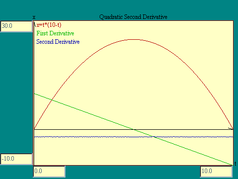
The series of at the left shows that the second derivative of the quadratic function is a straight line at a constant x=-2. The display from which this image was taken is the
Quadratic Second Derivative
display.
|
|
Just to round out this discussion of the rate of change of one
variable with respect to another let's consider the
derivative of two more functions. First the
sinusoidal function.
Run the
Sinusoidal Derivative
display to get an idea of the shape of the derivative curve.
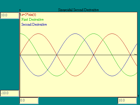
Notice that the sine function and its derivative have the same
cyclic shape only the derivative lags the sine by a quarter
cycle. You may, depending on your recollection of trigonometry,
recognize the derivative of the sine function as the
cosine
function. In any event that is what it is.
The second derivative of the sine function is just the original function with its sign reversed, or 180 degrees out of phase, which amounts to the same thing. The display from which the image at the right was taken is the
Sinusoidal Second Derivative
display.
|
|
|
Next take a look at the
Gaussian Derivative
display.
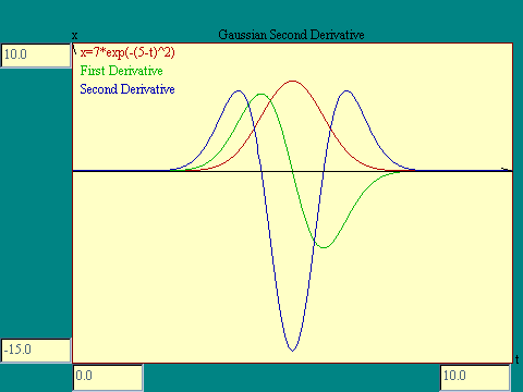
The second derivative of the Gaussian function is plotted in the
Gaussian Second Derivative
display.

Remember I warned you that we would have to deal with some
fundamentals whose application was not immediately obvious. Well
here we are introducing exotic stuff like second derivatives of
purely mathematical functions, not the sort of thing you probably
want to think about. So take a break and think about something
else for a while. These ideas will come back again when we begin
poking around in the laws of nature.

Are there any questions?
|

 Next
Next
 Previous
 Other
Other
|
|
|
|


